Intro
Every time you ask ChatGPT a question, get a movie recommendation on Netflix, or watch your phone recognize faces in photos, billions of matrix multiplications are happening behind the scenes. This fundamental mathematical operation has become the computational backbone of modern artificial intelligence.
GEMM (General Matrix Multiply) is the technical term for these matrix multiplication operations, and it’s no exaggeration to say that GEMM is omnipresent in machine learning. When a neural network predicts house prices using linear regression, it’s performing matrix multiplications to combine features and weights. When a recurrent neural network analyzes product review sentiment, GEMM operations process sequential data through hidden states. When a convolutional neural network generates captions for your Instagram photos, countless matrix operations extract and combine visual features.
The AI revolution from classic machine learning (pre-2010) through deep learning (2010s) to today’s generative AI era has been enabled by our ability to perform these matrix operations at unprecedented scale. Modern large language models like the ones powering ChatGPT, Gemini, and Claude require trillions of matrix operations for both training and inference. A single forward pass through GPT-3 for instance, involves matrix multiplications with dimensions in the thousands, repeated across 96 layers. While working on understanding Transformer architectures and implementing them in PyTorch, I initially took these operations for granted—calling torch.matmul() without considering what happens underneath. But when I began peeling the layers of abstraction in frameworks like PyTorch and TensorFlow, I discovered a fascinating world of optimization. The journey from a simple matrix multiplication to GPU-accelerated GEMM operations involves sophisticated decisions about memory hierarchies, thread management, and hardware utilization.
This curiosity led me to explore CUDA architecture and the specialized libraries (cuBLAS, cuDNN, CUTLASS) that PyTorch calls behind the scenes. In this blog series, I’ll take you through that same journey—from naive matrix multiplication to highly optimized GPU implementations. We’ll explore why simple approaches fail at scale, how tiled GEMM leverages GPU memory hierarchies, how Tensor Cores accelerate modern AI workloads, and how CUDA libraries abstract away the complexity of optimal GPU utilization.
This is just the tip of the iceberg, and as they say, the devil is in the details. But understanding these fundamentals will give you a new appreciation for the computational machinery powering today’s AI revolution.
Matrix Multiplication
Matrix Multiplication as we know has time complexity of O(N^3) , O(N^3) is not acceptable this definitely requires optimization, consider the scale of modern AI: a single attention mechanism in a large language model can involve large matrices and numerous matrix multipliations are involved across the layers of the models , If these core operations aren’t efficient even the most performant inference engines like vLLM or Triton can’t provide better results despite of the optimizations such as KV Cache, Prefill, Speculative Decoding etc…
The Computational Challenge
Let’s examine a concrete example. Consider multiplying two matrices: A (256×256) and B (256×256), resulting in matrix C (256×256).
To calculate any element C(i,j), we need to compute the dot product of row i from matrix A with column j from matrix B. For C(0,0), we multiply the first row of A with the first column of B and sum the results:
This requires 256 multiply-add operations. Since our result matrix has 256×256 = 65,536 elements, and each requires 256 operations, we need a total of 167,77,216 FMA (Fused Multiply-Add) operations.
The Naive Sequential Approach
The most straightforward implementation uses three nested loops: This sequential approach calculates elements one by one: C(0,0) → C(0,1) → … → C(255,255). On a modern CPU, this might take several seconds, which is unacceptable for real-time inference.
include visualization from Claude if possible
The Parallelization Opportunity
Here’s the key thing to observe, each element of the result matrix C can be calculated independently. Computing C(255,255) doesn’t depend on any previous calculations of matrix C. This independence is the foundation for parallelization. Theoretically, we could spawn 65,536 threads—one for each result element. Thread-0 calculates C(0,0), Thread-1 calculates C(0,1), and so on. If we could execute all threads simultaneously, our computation time would be determined by the maximum time to perform 256 FMA operations rather than 8+ million.
Analogy
Manufacturing Plant that produces Cars, it requires the Skilled Technicians for assembling the Parts , the Technicians require Parts & Tools to assemble them as single Unit (Car)
Though I mentioned that we can parallelize the whole process by creating multiple threads one for each element, this has some constraints , to understand these constraints we need to understand GPU Architecture, in the next section we will try to understand minimum terminology that lays foundation for understanding the GEMM and Optimizations at different levels.
GPU Architecture
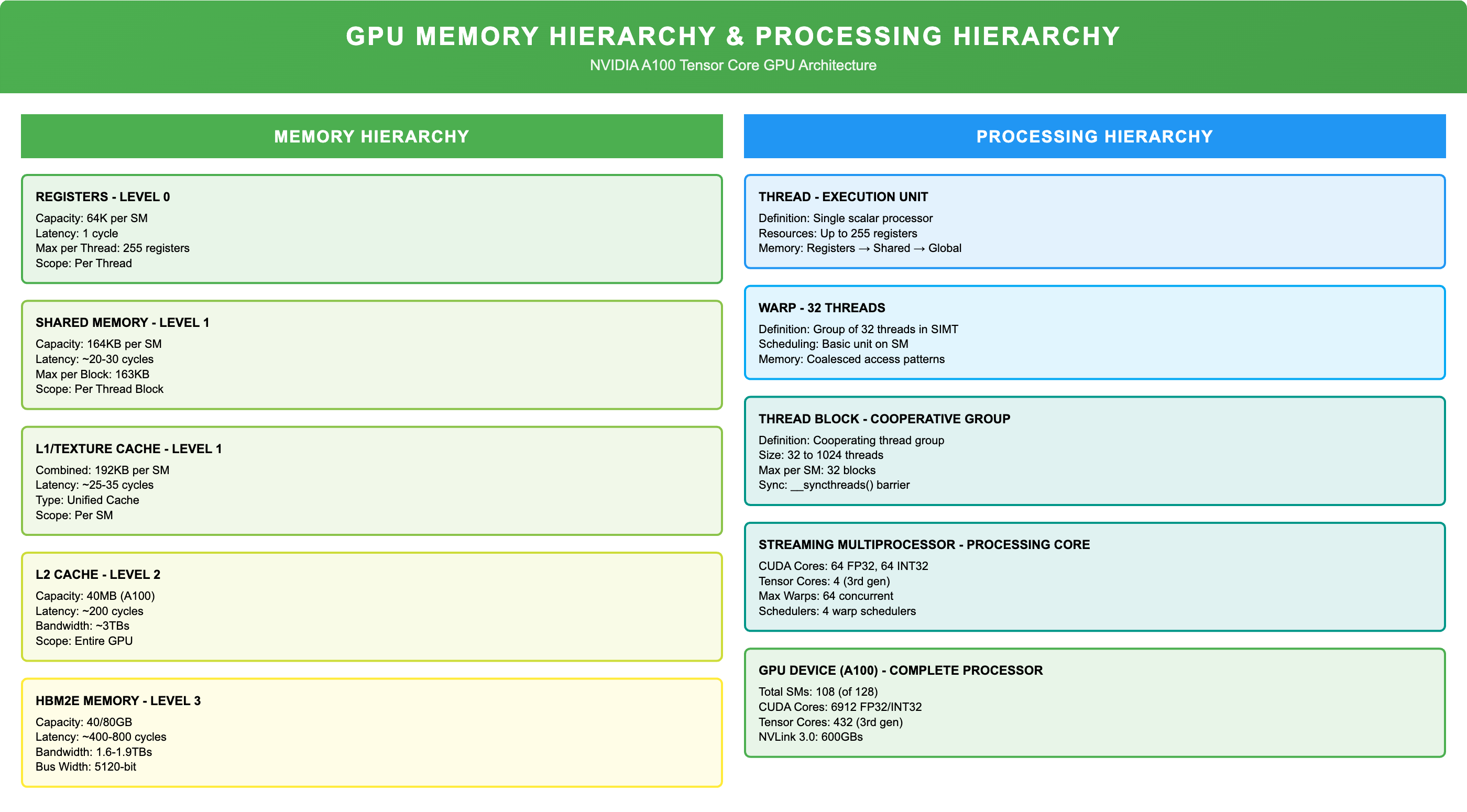
To optimize Matrix Multiplication for scale that is required for ML/AI workloads, we should have better understanding of GPU architecture, Processing & Memory hierarchies which are two corner stones for any GPU workload. Like a manufacturing plant producing cars has critical resources like Technicians, Tools, Raw Materials & and Place to keep all the required Parts. GPUs too have critical resources some of them are highlighted in below , while each NVIDIA GPU Architecture has lot of these configurations we are only touching few of the important configurations that are relevant in our context, we can find full architecture details for Ampere here
Processing Units (The Skilled Technicians):
- Threads: Individual workers
- Warps: Small coordinated group. of 32 threads
- Thread Blocks: Teams of workers assigned to Complete a task
- CUDA Cores/Tensor Cores: Individual workstations in a Workshop
- Streaming Multiprocessors (SMs): The main production lines where work gets done, think of each SM as Workshop
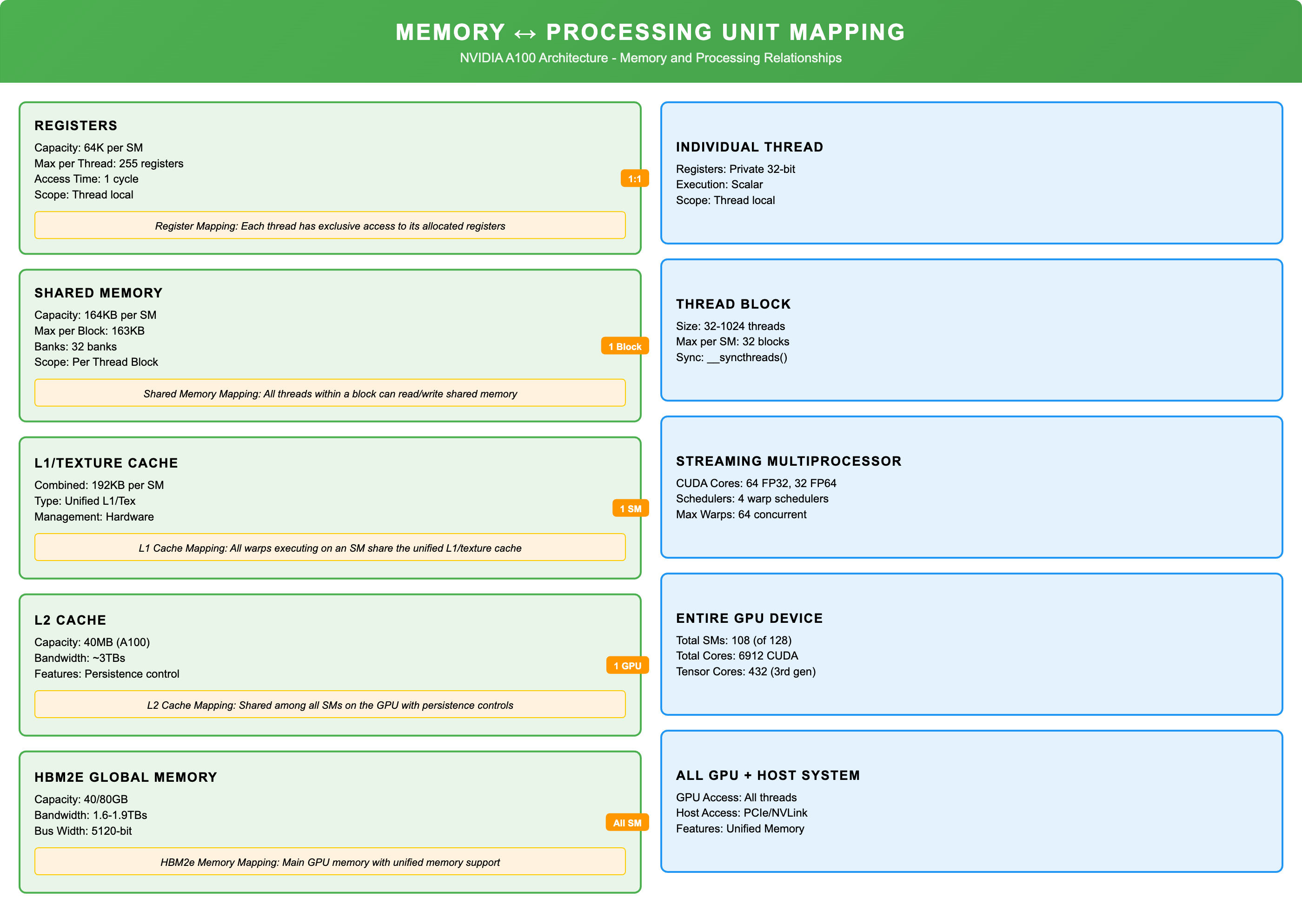
Memory Hierarchy (storage for parts and materials):
- Registers: immediate tools required for Technician (fastest, most limited)
- Shared Memory/L1 Cache: Workshop floor storage (fast but limited)
- L2 Cache: Regional storage - Shared across all SMs
- Global RAM: The main warehouse (large but distant)
Resource Constraints:
Just as our manufacturing plant has limited skilled technicians and Shop Floor space, GPUs have finite resources. For NVIDIA’s A100 (Ampere architecture), we have to be aware of these constrains before writing CUDA functions or kernels to achieve our objectives
-
108 Streaming Multiprocessors
-
2,048 maximum threads per SM
-
64 maximum Warps per SM
-
1024 Threads per Block
-
64 FP32 cores + 32 FP64 cores + 4 Tensor cores per SM
-
Total Threads = 2048 Threads per SM * 108 SM = 221,184 Threads per GPU
-
Global (HBM) memory: 40GB
-
L2 Cache: 40MB
-
Shared-memory+L1(Shared across Thread Block): 192KB
-
Maximum Shared-Memory Configurable: 164KB
-
Registers: 64K 32-bit Registers per SM, 255 Registers per Thread
CUDA Programming Terminology:
Kernel:
A kernel is a function that executes on the GPU to achieve our computational objective. In our manufacturing analogy, it’s the instruction manual that guides each technician on the steps to follow for their specific task.
For matrix multiplication, our kernel would contain the instructions for computing C[i][j] = A[i][k] * B[k][j] for assigned matrix elements.
Though the GPU performs the actual computation, the CPU orchestrates the entire process. The way I like to think about it is like maritime logistics where cargo is transferred to smaller vessels (lighters) before reaching the main ship: Before Kernel is launched on GPU, CPU copies the data to GPU HBM Memory(Global Memory)
- Declare Host Variables (Host = CPU)
- Declare Device Variables (Device = GPU)
- Allocate Device Memory (Memory to Store the Data Required in Global Memory HBM)
- Copy Host → Device (Transfer input data to GPU)
- Launch Kernel (Execute Main Function)
- Copy Device → Host (Retrieve results from GPU to CPU)
- Free Memory(Clean up alloacted memory)
Thread Hierarchy
To perform computations on the GPU, we write kernels, whether developing custom kernels or using existing ones, each kernel requires processing units (CUDA/Tensor cores) and memory resources for execution. These resources are orgaized according to configurations specified during kernel launch.
The resource allocation involves a two-tier responsibility model:
- Developer-controlled: Grid dimensions, Block dimensions, shared memory usage, Register Usate
- Hardware/scheduler-controlled: Warp Scheduling, Streaming Multiprocessor assignment, Instruction scheduling
Developer’s doesn’t specify individual threads directly. Instead number of required threads expressed through Grid & Thread Blocks configuration which uses a hierarchical approach: Grid → Thread Blocks → Warps → Threads, both Grids & Blocks configurations can be expressed using 1D,2D & 3D to address problem statements belonging to diffrent domains.
Warp
A critical aspect of CUDA’s execution model is the Warp - This is not controlled by developers. While we specify the grid and block dimensions, we don’t specify the warp size, which is controlled by schedulers and is constant at 32 threads per warp executed simultaneously.
An important note about warps is that even if we specify just 1 thread per block, the warp scheduler still allocates a full warp of 32 threads, with 31 threads remaining unused. This significantly impacts SM utilization and should be considered when designing kernel launch configurations. The table below shows the impact of thread block size on warp utilization.
| Thread Block Size | Warps Used | Warp Utilization |
|---|---|---|
| 16 Threads | 1 Warp | 50% (16/32) |
| 32 Threads | 2 Warps | 100% (32/32) |
| 48 Threads | 2 Warps | 75% (48/64) |
| 64 Threads | 2 Warps | 100% (64/64) |
| 96 Threads | 3 Warps | 100% (96/96) |
SIMT (Single Instruction Multiple Thread)
SIMT is the execution model used by CUDA kernels. Consider multiplying matrix A of size (256,256) by a constant C. The instruction A[i][j] = C * A[i][j] remains the same for all iterations except for the index values. This nested loop can be converted to execute in parallel, where each thread calculates one element on the GPU.
This is achieved by issuing the same instruction to a group of 32 threads (a warp), as discussed earlier. Though threads are the fundamental building blocks for GPU processing, instructions are issued at the warp level. Hence, when an instruction is issued, it’s executed by all active threads in the warp.
Note: In modern architectures, there are modifications where collections of threads work together on computations (like Thread Block Clusters), but this basic SIMT model covers the fundamental concept.
for i in range(256):
    for j in range(256):
        A[i][j] = C * A[i][j]
Grid Configuration
Grid Dimension (gridDim): The grid dimension specifies the number of blocks in the grid. It determines how many blocks are launched to execute the kernel.
Thread Block Configuration
Block Dimension (blockDim): The block dimension specifies the number of threads within a single block.
Kernel Launch
kernel<<<gridDim, blockDim>>>(parameters)
- Thread blocks per grid: 16 × 16 = 256 thread blocks
- Threads per block: 16 × 16 = 256 threads
- Warps per Block : 256 / 32 = 8 Warps per Block
- Total Warps : 8 * 256 = 2048 Warps
- Total threads: 256 × 256 = 65,536 threads
This is one possible configuration for processing a 256×256 matrix where each thread handles one matrix element(This is not Optimal configuration)
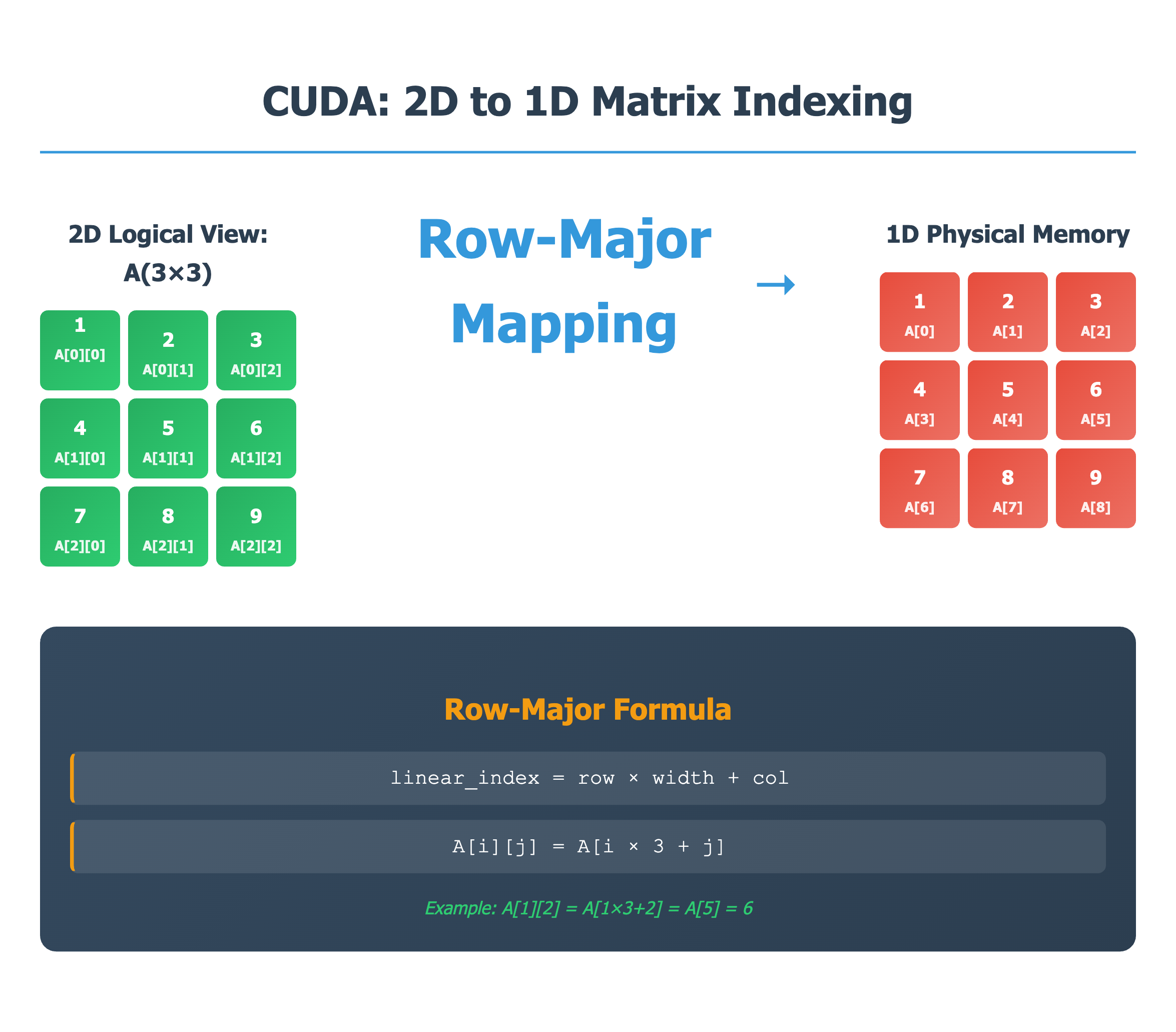
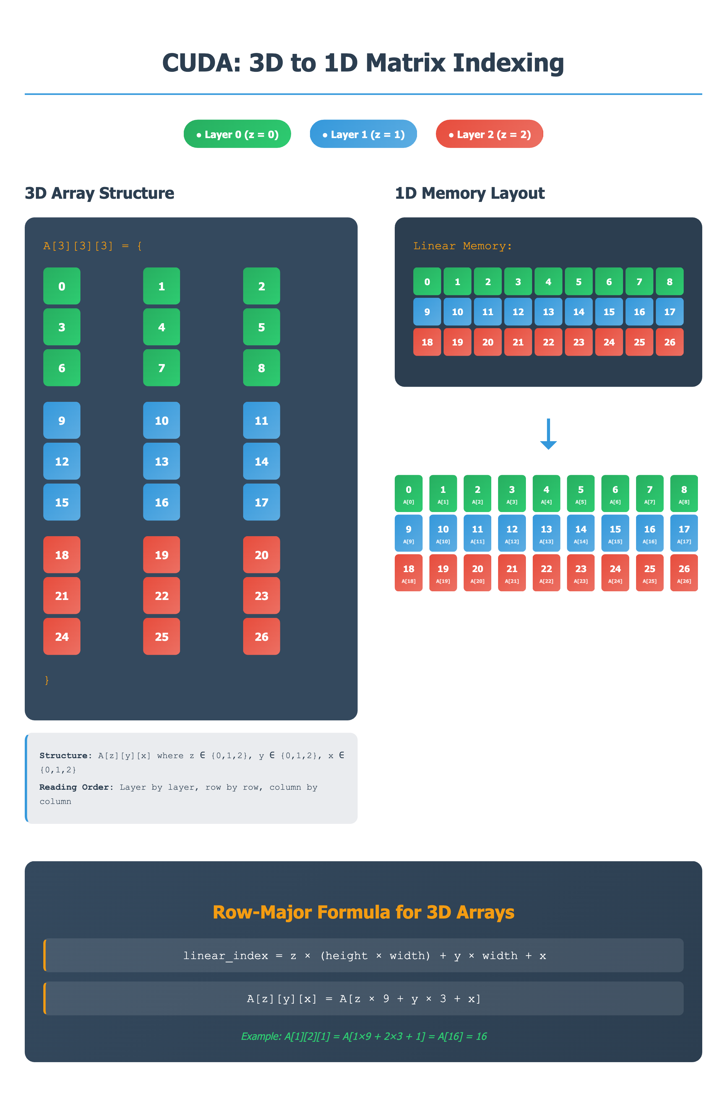
Logical vs Physical Representation
The above representation is logical representation , internally GPU operates on liner indexes, hence it would be converted to linear index, either the developer can do it or internally it is converted to linear index, below image gives idea on how to
- Linear thread IDs within each warp (32 consecutive threads)
- Linear memory addresses in global memory
- Sequential instruction execution within warps
thread Indexes are linear hence while accessing the elements of matrix we can use either of the representations either 2D or linear indexing below is one example of how 2D indexes can be converted to linear indexing.
Memory Coalescing : Efficient Data Access Patterns
The way matrix elements are stored in memory significantly impacts kernel performance. Understanding how threads access memory is crucial for achieving optimal GPU performance in matrix operations to avoid Kernels starving for data due to slow memory access.
GPU Memory Operations Overview
GPU memory operations can be categorized into three phases:
- Load - Transfer data from global memory to registers directly or via shared memory
- Compute - Execute the actual mathematical operations on data in registers
- Store operations - Write results back to global memory
The important point to consider is that memory bandwidth not computational power which often becomes the bottleneck in GPU kernels. This is why optimizing memory access patterns has significant role while writing custom CUDA Kernels.
Memory coalescing occurs when threads within the same warp access consecutive memory addresses. When this happens, the GPU can combine multiple memory requests into fewer, wider memory transactions, dramatically improving bandwidth utilization.
Note:- Coaelscing is determined by the access pattern of the 32 threads within a single warp, not by the overall grid structure.
Memory Storage Layouts
By default, C++ stores matrices in row-major layout while Fortran uses column-major layout. This is analogous to how databases can be organized as row-oriented (traditional RDBMS) or column-oriented (analytical databases) based on storage patterns.

Whether we are using CPU or GPU for computation, data first needs to be brought to execution units ALU in CPU or CUDA Cores in GPU which is accomplished using Load instruction , Upon load instruction data is moved from Global Memory to Registers either directly or through Shared Memory , Registers are High speed memory . to keep it simple for our discussion each Load instruction can only access certain number of bytes in one cycle, when all of our threads in a Warp are accessing adjacent locations one load instruction can fetch all the inputs required for a threads in Warp to be processed , If the threads of the same Warp are accessing the elements that are distant that leads to multiple load instructions from Global Memory which is time taking process as transfer of data from Global Memory is constrained by the bandwidth , because CUDA cores complete the instructions and waits for the data while the load instruction still fetching the data from Global Memory, hence it is paramount important to make sure the data should be arranged such that threads in a warp access consectutive elements for thier respective operations.
Analogy:
In our Manufacturing analogy, if all the technicians are working on same part of Car, all the technicians require parts from same bin or near by Bins , one supply truck make a single trip to to load all parts from consecutive bins, otherwise if each technician is working on different part of car which requires part from different bins this makes it difficult to load all parts from different bins , this might require multiple iterations to bring parts required for all technicians , which impacts the overall execution of the manufacturing process
Let us go through some examples of Coalesce and Non-Coalesce patterns to understand this better
Coalesced Memory Access Pattern Example
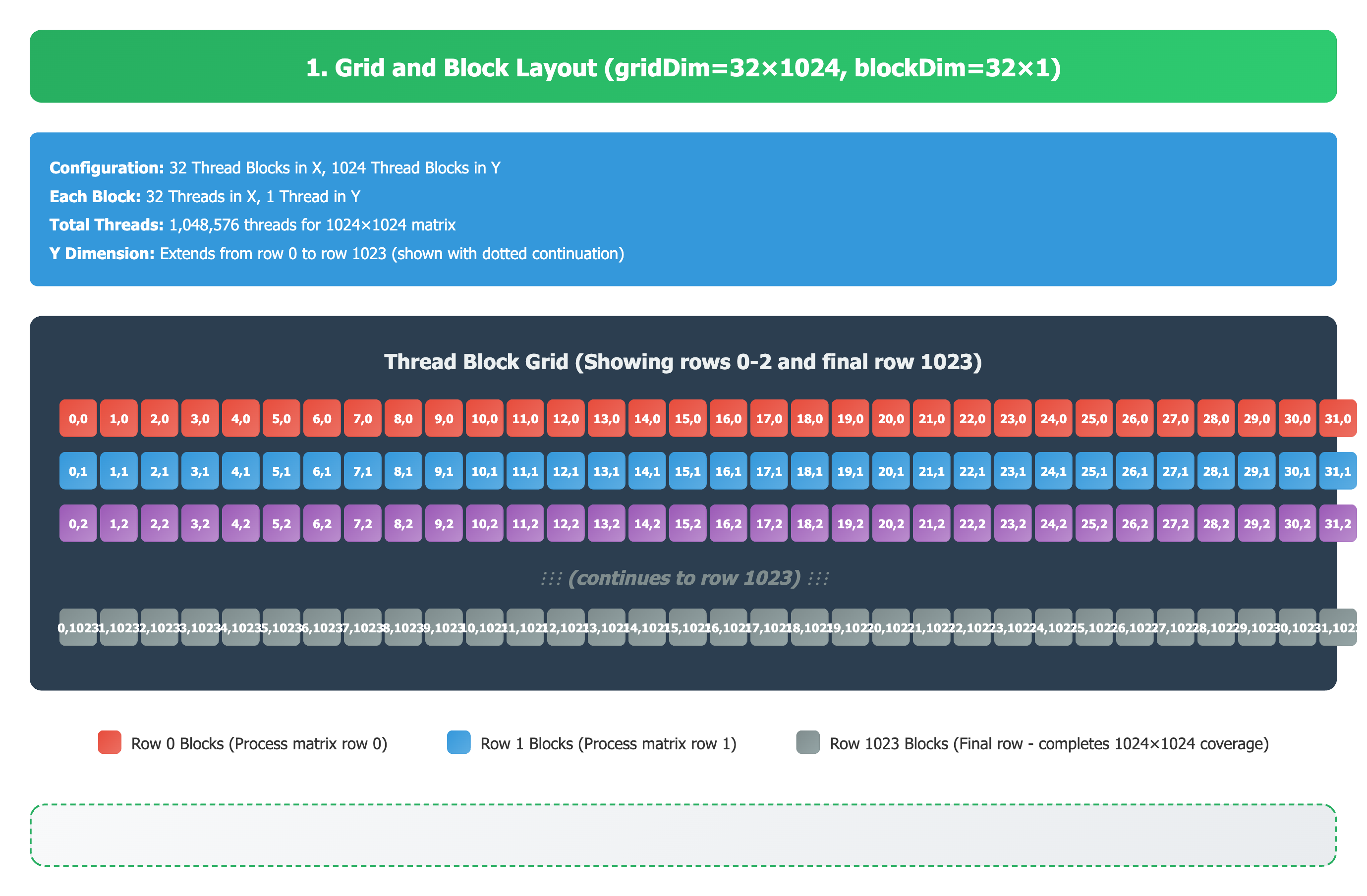
Consider matrix multiplication for matrices A=(1024×1024), B=(1024×1024), C=(1024×1024) using a configuration that results in optimal coalesced memory access.
Configuration Parameters
Thread Block Organization
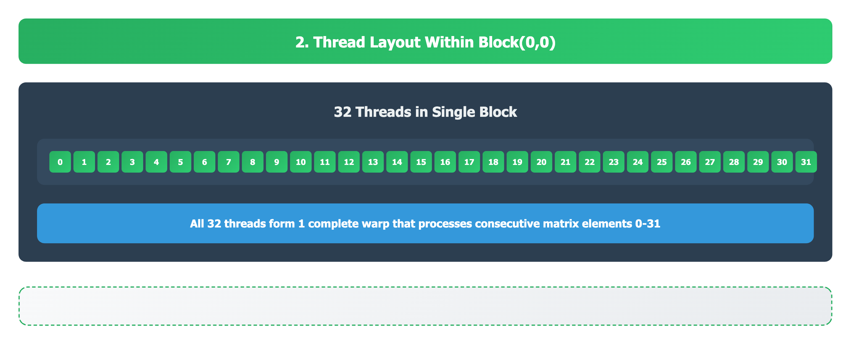
Thread Organization within Each Block
Linear Index Calculation Formula
Coalesced Memory Access Analysis
Perfect Coalescing: Each Warp Accesses Consecutive Memory
With blockDim(32,1), each warp contains 32 threads that access 32 consecutive memory locations within the same matrix row.
Coaelsced Visulizations


Thread Block (0,0) - Complete Warp Analysis:
Thread 0:
Parameters: blockIdx.x=0, blockIdx.y=0, threadIdx.x=0, threadIdx.y=0

Calculation:
row = 0 * 1 + 0 = 0
col = 0 * 32 + 0 = 0
idx = 0 * 1024 + 0 = 0
Thread 1:
Parameters: blockIdx.x=0, blockIdx.y=0, threadIdx.x=1, threadIdx.y=0

Calculation:
row = 0 * 1 + 0 = 0
col = 0 * 32 + 1 = 1
idx = 0 * 1024 + 1 = 1
Thread 2:
Parameters: blockIdx.x=0, blockIdx.y=0, threadIdx.x=2, threadIdx.y=0

Calculation:
row = 0 * 1 + 0 = 0
col = 0 * 32 + 2 = 2
idx = 0 * 1024 + 2 = 2
…continuing pattern…
Thread 31:
Parameters: blockIdx.x=0, blockIdx.y=0, threadIdx.x=31, threadIdx.y=0

Calculation:
row = 0 * 1 + 0 = 0
col = 0 * 32 + 31 = 31
idx = 0 * 1024 + 31 = 31
✅ Perfect Coalescing: All 32 threads access consecutive indices 0, 1, 2, …, 31
Thread Block (1,0) - Next Consecutive Block:
Thread 0:
Parameters: blockIdx.x=1, blockIdx.y=0, threadIdx.x=0, threadIdx.y=0

Calculation:
row = 0 * 1 + 0 = 0
col = 1 * 32 + 0 = 32
idx = 0 * 1024 + 32 = 32
Thread 1:
Parameters: blockIdx.x=1, blockIdx.y=0, threadIdx.x=1, threadIdx.y=0

Calculation:
row = 0 * 1 + 0 = 0
col = 1 * 32 + 1 = 33
idx = 0 * 1024 + 33 = 33
…continuing pattern…
Thread 31:
Parameters: blockIdx.x=1, blockIdx.y=0, threadIdx.x=31, threadIdx.y=0

Calculation:
row = 0 * 1 + 0 = 0
col = 1 * 32 + 31 = 63
idx = 0 * 1024 + 63 = 63
✅ Perfect Coalescing: All 32 threads access consecutive indices 32, 33, 34, …, 63
Thread Block (31,0) - Final Block in Row 0:
Thread 0:
Parameters: blockIdx.x=31, blockIdx.y=0, threadIdx.x=0, threadIdx.y=0

Calculation:
row = 0 * 1 + 0 = 0
col = 31 * 32 + 0 = 992
idx = 0 * 1024 + 992 = 992
Thread 1:
Parameters: blockIdx.x=31, blockIdx.y=0, threadIdx.x=1, threadIdx.y=0

Calculation:
row = 0 * 1 + 0 = 0
col = 31 * 32 + 1 = 993
idx = 0 * 1024 + 993 = 993
…continuing pattern…
Thread 31:
Parameters: blockIdx.x=31, blockIdx.y=0, threadIdx.x=31, threadIdx.y=0

Calculation:
row = 0 * 1 + 0 = 0
col = 31 * 32 + 31 = 1023
idx = 0 * 1024 + 1023 = 1023
✅ Perfect Coalescing: All 32 threads access consecutive indices 992, 993, 994, …, 1023
Summary: Coalesced Access Pattern
| Thread Block | Memory Indices Accessed | Pattern | Gap Size |
|---|---|---|---|
| Block (0,0) | 0, 1, 2, …, 31 | ✅ Consecutive | 0 |
| Block (1,0) | 32, 33, 34, …, 63 | ✅ Consecutive | 0 |
| Block (2,0) | 64, 65, 66, …, 95 | ✅ Consecutive | 0 |
| … | … | ✅ Consecutive | 0 |
| Block (31,0) | 992, 993, 994, …, 1023 | ✅ Consecutive | 0 |
Key Advantages
- No Memory Gaps: Every thread in a warp accesses consecutive memory addresses
- Single Memory Transaction: Each warp requires only 1 memory transaction
- Optimal Bandwidth Utilization: 100% of memory bandwidth is effectively used
- Maximum Performance: Optimal memory access pattern for GPU architecture
Warp-Level Analysis
Since each thread block contains exactly 32 threads = 1 warp:
| Thread Block | Warp | Threads | Memory Access Pattern |
|---|---|---|---|
| Block (0,0) | Warp 0 | 0-31 | Consecutive: 0-31 ✅ |
| Block (1,0) | Warp 0 | 0-31 | Consecutive: 32-63 ✅ |
| Block (2,0) | Warp 0 | 0-31 | Consecutive: 64-95 ✅ |
| … | … | … | … |
| Block (31,0) | Warp 0 | 0-31 | Consecutive: 992-1023 ✅ |
Why This Configuration Works
- blockDim.y = 1: Ensures all threads in a warp stay within the same matrix row
- blockDim.x = 32: Matches warp size, providing optimal thread-to-warp mapping
- Consecutive Access: ThreadIdx.x directly maps to consecutive column indices
- No Row Spanning: Warps never span multiple matrix rows, eliminating gaps
Key Insight: The fundamental success of blockDim(32,1) is that it aligns perfectly with GPU Warp architecture, ensuring each warp accesses a single contiguous block of memory within the same matrix row.
Non-Coalesced Memory Access Pattern Example
Consider matrix multiplication for matrices A=(1024×1024), B=(1024×1024), C=(1024×1024) using a configuration that results in non-coalesced memory access.
Configuration Parameters
gridDim = (64,64)   => 64 Thread Blocks in X dimension, 64 Thread Blocks in Y dimension
blockDim = (16,16)  => 16 Threads in X dimension, 16 Threads in Y dimension

gridDim.x = 64      blockDim.x = 16
gridDim.y = 64      blockDim.y = 16

threadIdx.x range: 0-15    blockIdx.x range: 0-63
threadIdx.y range: 0-15    blockIdx.y range: 0-63
Total Configuration:
- Total Thread Blocks: 64 × 64 = 4,096 blocks
- Total Threads per Block: 16 × 16 = 256 threads
- Total Warps per Block: 256 ÷ 32 = 8 warps
- Total Threads: 1,048,576 threads (perfect for 1024×1024 matrix)
Thread Block Organization
Thread Block Layout (64×64 grid):

Thread Block (0,0)    Thread Block (1,0)    Thread Block (2,0)    ...    Thread Block (63,0)
Thread Block (0,1)    Thread Block (1,1)    Thread Block (2,1)    ...    Thread Block (63,1)
Thread Block (0,2)    Thread Block (1,2)    Thread Block (2,2)    ...    Thread Block (63,2)
.
.
.
Thread Block (0,63)   Thread Block (1,63)   Thread Block (2,63)   ...    Thread Block (63,63)
Thread Organization within Each Block
Thread Layout (16×16 per block):

threadIdx(0,0)    threadIdx(1,0)    threadIdx(2,0)    ...    threadIdx(15,0)
threadIdx(0,1)    threadIdx(1,1)    threadIdx(2,1)    ...    threadIdx(15,1)
threadIdx(0,2)    threadIdx(1,2)    threadIdx(2,2)    ...    threadIdx(15,2)
.
.
.
threadIdx(0,15)   threadIdx(1,15)   threadIdx(2,15)   ...    threadIdx(15,15)
Linear Index Calculation Formula
row = blockIdx.y * blockDim.y + threadIdx.y
col = blockIdx.x * blockDim.x + threadIdx.x
idx = row * matrix_width + col    (where matrix_width = 1024)
Non-Coalesced Memory Access Analysis
Non-Coelesced Visulizations
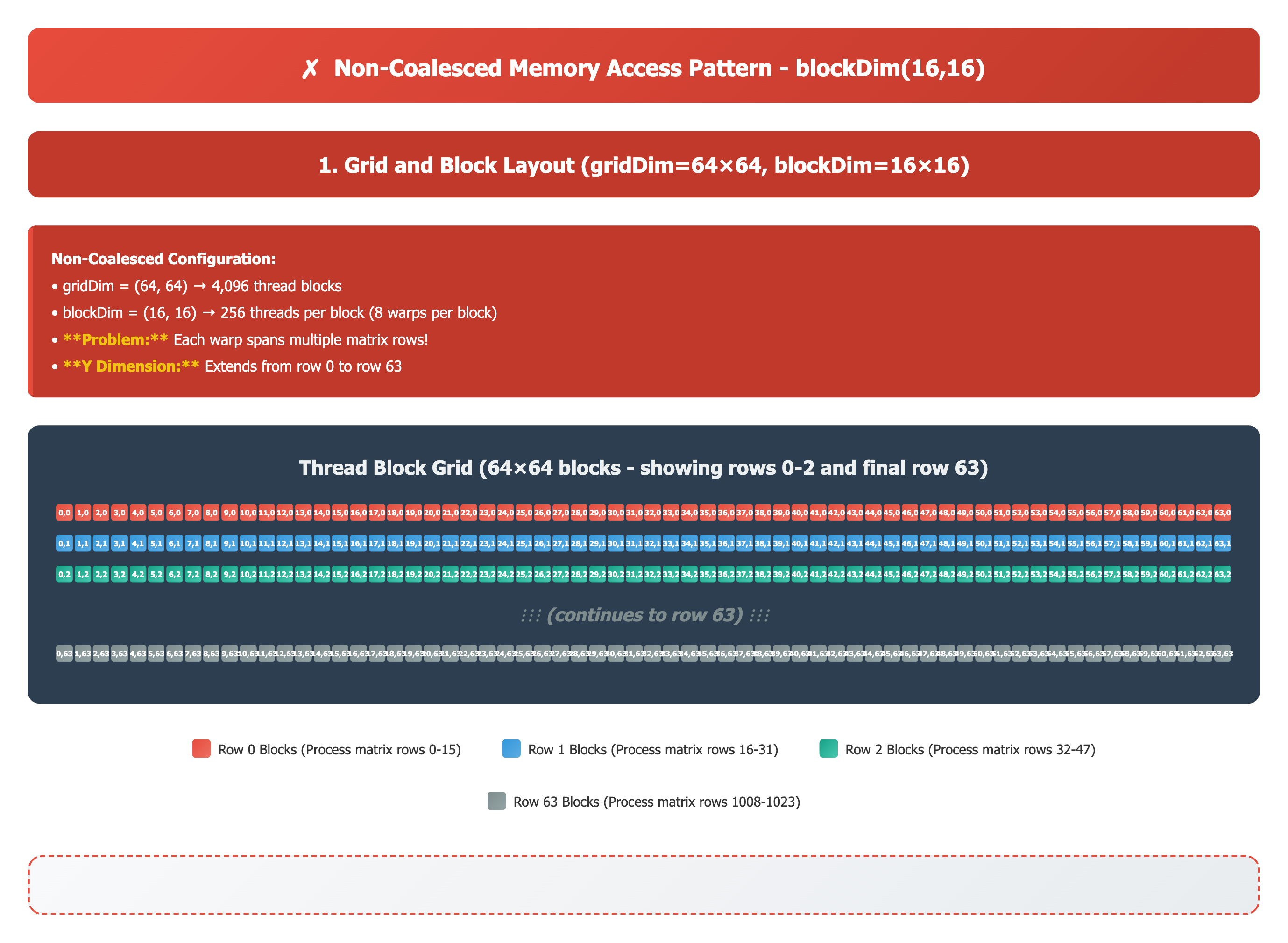
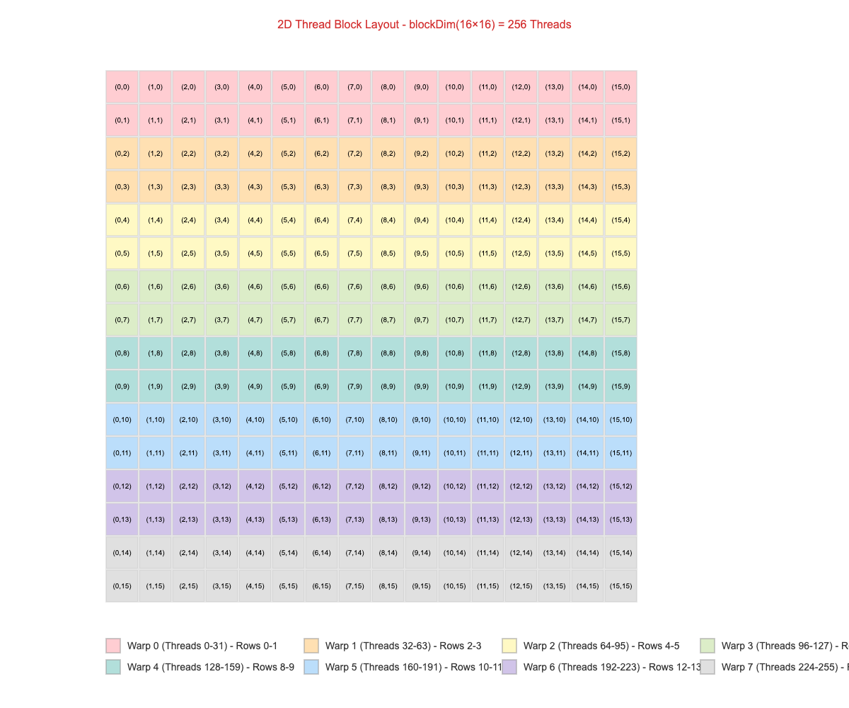
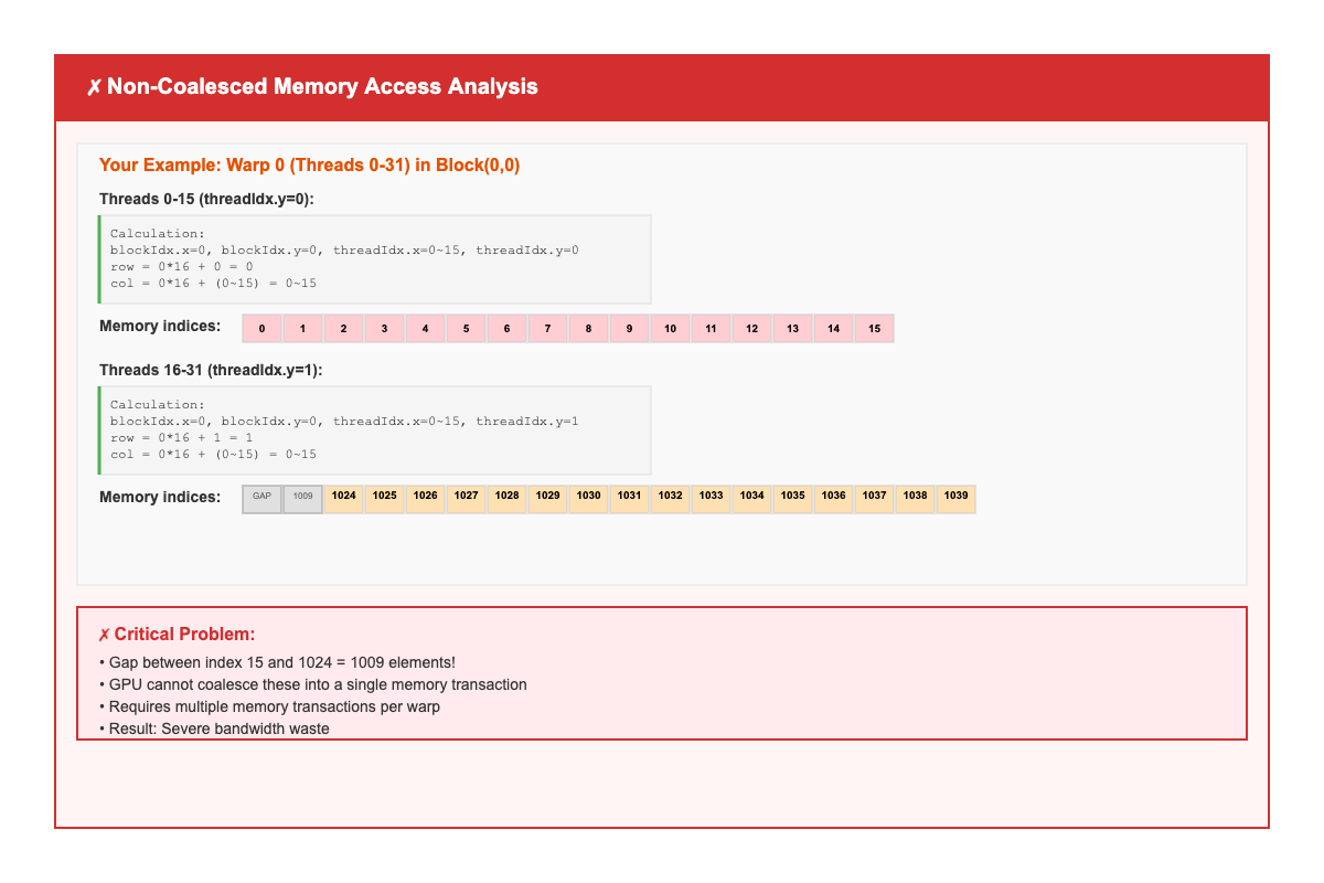
Problem: Warps Span Multiple Matrix Rows
With blockDim(16,16), each warp contains 32 consecutive threads that span 2 matrix rows, creating large memory gaps.
Warp 0 (Threads 0-31) in Thread Block (0,0):
First 16 threads (threadIdx.y = 0):
Parameters: blockIdx.x=0, blockIdx.y=0, threadIdx.x=0-15, threadIdx.y=0

Calculation:
row = 0 * 16 + 0 = 0
col = 0 * 16 + (0-15) = 0-15
idx = 0 * 1024 + (0-15) = 0-15

Memory indices accessed: 0, 1, 2, 3, ..., 14, 15
Next 16 threads (threadIdx.y = 1):
Parameters: blockIdx.x=0, blockIdx.y=0, threadIdx.x=0-15, threadIdx.y=1

Calculation:
row = 0 * 16 + 1 = 1
col = 0 * 16 + (0-15) = 0-15
idx = 1 * 1024 + (0-15) = 1024-1039

Memory indices accessed: 1024, 1025, 1026, ..., 1038, 1039
❌ Gap Analysis: 1009 elements between indices 15 and 1024!
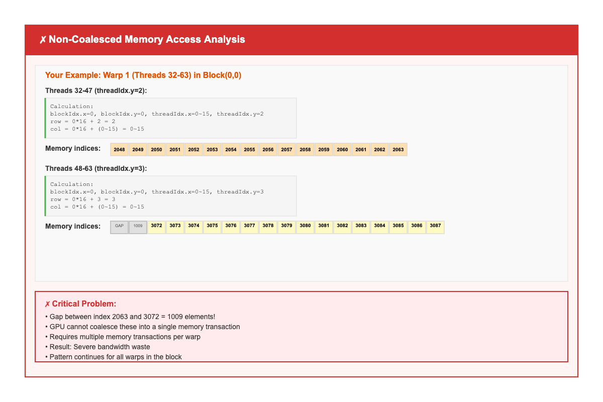
Warp 1 (Threads 32-63) in Thread Block (0,0):
Threads 32-47 (threadIdx.y = 2):
Parameters: blockIdx.x=0, blockIdx.y=0, threadIdx.x=0-15, threadIdx.y=2

Calculation:
row = 0 * 16 + 2 = 2
col = 0 * 16 + (0-15) = 0-15
idx = 2 * 1024 + (0-15) = 2048-2063

Memory indices accessed: 2048, 2049, 2050, ..., 2062, 2063
Threads 48-63 (threadIdx.y = 3):
Parameters: blockIdx.x=0, blockIdx.y=0, threadIdx.x=0-15, threadIdx.y=3

Calculation:
row = 0 * 16 + 3 = 3
col = 0 * 16 + (0-15) = 0-15
idx = 3 * 1024 + (0-15) = 3072-3087

Memory indices accessed: 3072, 3073, 3074, ..., 3086, 3087
❌ Same Gap Problem: 1009 elements between indices 2063 and 3072!
Final Warp Example - Warp 7 (Threads 224-255):
Threads 224-239 (threadIdx.y = 14):
Parameters: blockIdx.x=0, blockIdx.y=0, threadIdx.x=0-15, threadIdx.y=14

Calculation:
row = 0 * 16 + 14 = 14
col = 0 * 16 + (0-15) = 0-15
idx = 14 * 1024 + (0-15) = 14336-14351
Threads 240-255 (threadIdx.y = 15):
Parameters: blockIdx.x=0, blockIdx.y=0, threadIdx.x=0-15, threadIdx.y=15

Calculation:
row = 0 * 16 + 15 = 15
col = 0 * 16 + (0-15) = 0-15
idx = 15 * 1024 + (0-15) = 15360-15375
Summary: Non-Coalesced Access Pattern
| Warp | First 16 Threads Access | Next 16 Threads Access | Gap Size | Coalesced? |
|---|---|---|---|---|
| Warp 0 | 0-15 (row 0) | 1024-1039 (row 1) | 1009 elements | ❌ No |
| Warp 1 | 2048-2063 (row 2) | 3072-3087 (row 3) | 1009 elements | ❌ No |
| Warp 2 | 4096-4111 (row 4) | 5120-5135 (row 5) | 1009 elements | ❌ No |
| … | … | … | 1009 elements | ❌ No |
| Warp 7 | 14336-14351 (row 14) | 15360-15375 (row 15) | 1009 elements | ❌ No |
Critical Problems
- Large Memory Gaps: Every warp has a 1009-element gap between consecutive thread accesses
- Multiple Memory Transactions: Each warp requires 2-4 separate memory transactions instead of 1
- Poor Bandwidth Utilization: Only 25-50% of memory bandwidth is effectively used
- Performance Degradation: 2-4x slower compared to coalesced access patterns
Key Insight: The fundamental issue with blockDim(16,16) is that it forces warps to span multiple matrix rows, breaking the consecutive memory access pattern required for optimal coalescing.
Compute vs Memory Bound Kernels
GPU kernels can be classified as either memory bound or compute bound based on their primary performance bottleneck. Understanding this classification is crucial for choosing the right optimization approach.
Like every computing system, GPUs have two fundamental dimensions: execution capability and memory bandwidth. Every system has scaling limits, and to improve performance, we can optimize along either dimension until reaching the maximum limits.
Key Classification Metric: Arithmetic Intensity
The fundamental metric for classification is Arithmetic Intensity:
background-color: #ffffff;
color: #2d2d2d;
padding: 16px;
margin: 0;
font-size: 15px;
line-height: 1.5;
overflow-x: auto;
“> Arithmetic Intensity = FLOPs (Floating Point Operations) / Bytes Accessed
Peak Arithemtic Intensity for A100 = 9.75 FLOP/byte
Above 9.75 FLOP/byte: Compute-bound(can potentially use full 19.5 TFLOPS)
Below 9.75 FLOP/byte: Memory-bound (limited by 2.0 TB/s bandwidth)
Kernel Classification Definitions
Compute Bound Kernels
Definition: A kernel is compute-bound when its performance is limited by the speed of its mathematical operations. The GPU’s compute units (CUDA Cores, Tensor Cores) are the primary bottleneck, and their utilization is the limiting factor.
Optimization Strategies:
To optimize compute-bound kernels, the focus is on maximizing the efficiency of mathematical operations. This involves:
- Ensuring High Occupancy: Launching enough threads to fully saturate the GPU’s Streaming Multiprocessors (SMs) and keep the compute units busy.
- Leveraging Specialized Hardware: Using specialized cores like Tensor Cores for matrix multiplication.
- Multi-GPU Scaling: For workloads that exceed a single GPU’s capacity, distributing the work across multiple GPUs can
- Trade-off: Multi-GPU comes with data transfer overhead dependent on network bandwidth
Memory Bound Kernels
Definition:A kernel is memory-bound when its performance is limited by the speed at which data can be transferred to and from the GPU’s memory. The primary bottleneck is memory bandwidth.
Key Indicators:
- Low Compute Utilizaion (cores are idle, waiting for data).
- Poor cache hit rates
- High memory access latency
- Memory access inefficiencies (poor coalescing, cache thrashing)
Optimization Strategies:
To optimize memory-bound kernels, the focus is on reducing the amount of data transferred from high-latency memory and improving access patterns. This is achieved by:
- Maximize data reuse: Keep frequently accessed data in faster memory levels
- Optimize access patterns: Ensuring memory accesses are coalesced to reduce the number of memory transactions
- Use memory hierarchy efficiently: Thread Registers → L1 Cache/Shared Memory → L2 Cache → Global Memory (HBM2)
- Use lower precision: Mixed precision or reduced precision where high accuracy isn’t critical
Upcoming: The performance of a naive GEMM kernel is limited by memory bandwidth. The upcoming sections will show how using shared memory with tiling increases data reuse and reduces expensive round trips to global memory. This allows data to be reused on-chip and makes the kernel’s performance dependent on the speed of its mathematical operations, effectively making it compute-bound.